
By Paul V. Desanker | April 6, 27274
R and the Tidyverse: next steps using WB data by Stéphane Guillou
This document is redacted in R Markdown; the source file is available here: https://gitlab.com/stragu/DSH/blob/master/R/tidyverse_next_steps/tidyverse_next_steps.Rmd It is then knitted as a markdown file, which is the best version to view online and to print: https://gitlab.com/stragu/DSH/blob/master/R/tidyverse_next_steps/tidyverse_next_steps.md PD: see video at https://www.youtube.com/watch?v=2TZYeFcJQIk
Setting up
If you want to review the installation instructions: https://gitlab.com/stragu/DSH/blob/master/R/Installation.md
- If you are using your own laptop please open RStudio
- Make sure you have a working Internet connection
- On the Library’s training computers:
- Log in with your UQ username and password
- Make sure you have a working Internet connection
- Open the ZENworks application
- Look for “RStudio”
- Double click on RStudio, which will install both R and RStudio
With RStudio open, let’s make sure we have the necessary packages installed by running this command (this might take a few minutes):
install.packages("tidyverse")This will install the 8 core Tidyverse packages (and their dependencies).
What are we going to learn?
tidyr and purrr, just like dplyr and ggplot2, are core to the Tidyverse.
- tidyr can be used to tidy your data
- purrr is useful to apply functions iteratively on lists or vectors
Create a project and a script
Use the project menu (top right) to create a “New project…”. Let’s name this one “tidyverse”.
We also want to work more comfortably by typing our code in a script. You can use the new file dropdown menu, or Ctrl+Shift+N, and save your script as “process.R” in the current working directory.
Load the necessary packages
We can use one single command to load the core Tidyverse packages:
library(tidyverse)## -- Attaching packages --------------------------------------- tidyverse 1.3.1 --## v ggplot2 3.3.3 v purrr 0.3.4
## v tibble 3.1.0 v dplyr 1.0.5
## v tidyr 1.1.3 v stringr 1.4.0
## v readr 1.4.0 v forcats 0.5.1## Warning: package 'tibble' was built under R version 4.0.5## -- Conflicts ------------------------------------------ tidyverse_conflicts() --
## x dplyr::filter() masks stats::filter()
## x dplyr::lag() masks stats::lag()Tidy data
Tidy data makes it easy to transform and analyse data in R (and many other tools). Tidy data has observations in rows, and variables in columns. The whole Tidyverse is designed to work with tidy data.
Often, a dataset is organised in a way that makes it easy for humans to read and populate. This is called wide format. Tidy data is usually in “long” format.
The ultimate rules of tidy data are:
- Each row is an observation
- Each column is a variable
- Each cell contains one single value
Import data
We are using a dataset from the World Bank.
Let’s download the file:
# download data, save locally
download.file(url = "https://gitlab.com/stragu/DSH/raw/master/R/tidyverse_next_steps/data_wb_climate.csv",
              destfile = "data_wb_climate.csv")
… and read the data into an object:
# read CSV into an object
#climate_raw <- read_csv("data_wb_climate.csv",
#                    na = "..")
climate_raw <- read_csv("https://gitlab.com/stragu/DSH/raw/master/R/tidyverse_next_steps/data_wb_climate.csv",
                    na = "..")
##
## -- Column specification --------------------------------------------------------
## cols(
## .default = col_double(),
## `Country code` = col_character(),
## `Country name` = col_character(),
## `Series code` = col_character(),
## `Series name` = col_character(),
## `2011` = col_logical()
## )
## i Use `spec()` for the full column specifications.We defined with the na argument that, in this dataset, missing data is recorded as “..”.
You can use View() to explore your dataset. We can see that it doesn’t respect the tidy data principles in a couple of ways, the most obvious one being that different years are spread out between different columns.
Reshaping data
Lengthening
To go from wide format to long format, we can use the tidyr function pivot_longer(). Here, we want to gather all the columns titled with a year: we store the data in a “value” variable, and the years in a “year” variable.
climate_long <- pivot_longer(climate_raw,
                             `1990`:`2011`,
                             names_to = "year",
                             values_to = "value") %>%
  mutate(year = as.integer(year))
We add a mutate() step to convert the years from character to integers.
This is better, but there is still an issue: our value variable contains many different indicators.
Widening
To do the opposite, going from long to wide format, we can use the pivot_wider() function.
We have single observations spread across several rows, so we should spread the “value” column.
First, let’s keep a record of the correspondence between long descriptive variable names and their “code”, for later reference:
codes <- unique(climate_long[,c("Series code", "Series name")])
codes
## # A tibble: 5 x 2
## `Series code` `Series name`
## <chr> <chr>
## 1 EG.USE.COMM.GD.PP.KD Energy use per units of GDP (kg oil eq./$1,000 of 2005 P~
## 2 EG.USE.PCAP.KG.OE Energy use per capita (kilograms of oil equivalent)
## 3 EN.ATM.CO2E.KT CO2 emissions, total (KtCO2)
## 4 EN.ATM.CO2E.PC CO2 emissions per capita (metric tons)
## 5 EN.ATM.CO2E.PP.GD.KD CO2 emissions per units of GDP (kg/$1,000 of 2005 PPP $)This will be our key to variable details, or “code book”, for future reference.
Now, let’s widen the data (and remove some useless columns with dplyr::select()):
climate_tidy <- climate_long %>%
  select(-`Series name`, -SCALE, -Decimals) %>%
  pivot_wider(names_from = `Series code`,
              values_from = value)
Challenge 1
Have a look at this block of code. What do you think it does?
groups <- c("Europe & Central Asia",
            "East Asia & Pacific",
            "Euro area",
            "High income",
            "Lower middle income",
            "Low income",
            "Low & middle income",
            "Middle income",
            "Middle East & North Africa",
            "Latin America & Caribbean",
            "South Asia",
            "Small island developing states",
            "Sub-Saharan Africa",
            "Upper middle income",
            "World")
climate_tidy <- climate_tidy %>%
  filter(!`Country name` %in% groups)
Turns out this dataset contains grouped data as well as unique countries. Here, we created a list of grouped countries, and removed them from the data by using dplyr’s filter() function (inverting the filter with !).
We can now check that we’ve only got single countries left:
unique(climate_tidy$`Country name`)Visualising
Now that we have clean, tidy data, we can process and visualise our data more comfortably! For example, to visualise the increase in KT of CO2 for each country:
climate_tidy %>%
  ggplot(aes(x = year,
             y = EN.ATM.CO2E.KT,
             group = `Country name`)) +
  geom_line()
## Warning: Removed 1091 row(s) containing missing values (geom_path).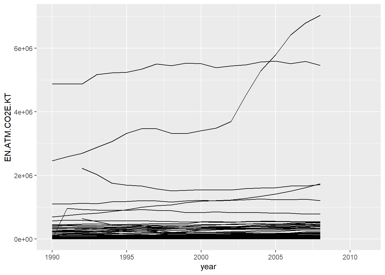
Let’s have a look at the increase in global CO2 emissions in KT:
climate_tidy %>%
  group_by(year) %>%
  summarise(CO2 = sum(EN.ATM.CO2E.KT, na.rm = TRUE)) %>%
  ggplot(aes(x = year, y = CO2)) +
  geom_point()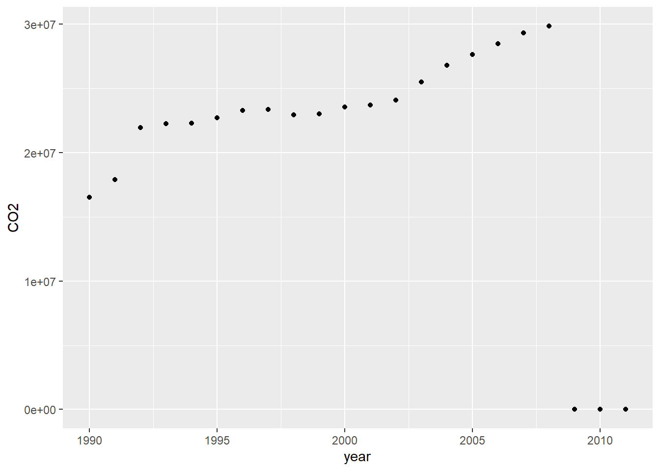
Challenge 2
Looks like our data is missing after 2008, so how can we remove that?
We can add this extra step:
climate_tidy %>%
  group_by(year) %>%
  summarise(CO2 = sum(EN.ATM.CO2E.KT, na.rm = TRUE)) %>%
  filter(year < 2009) %>%
  ggplot(aes(x = year, y = CO2)) +
  geom_point()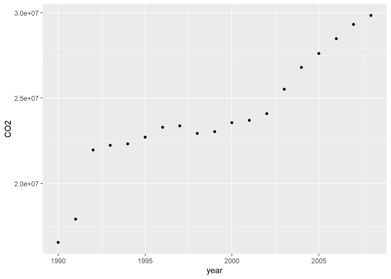
Functional programming
Functional programming (as opposed to “imperative programming”) makes use of functions rather than loops to iterate over objects. The functions will allow to simplify our code, by abstracting common building blocks used in different cases of iteration. However, it means that there will usually be a different function for each different pattern.
You can iterate over elements by using:
- the basic building blocks in R (for loops, while loops…), or
- the
applyfunction family from base R, or - the purrr functions.
Imagine we want to find out the median value for each variable in the mtcars dataset. Here is an example of a for loop:
output <- vector("double", ncol(mtcars))
for (i in seq_along(mtcars)) {
  output[[i]] <- median(mtcars[[i]])
}
output
## [1] 19.200 6.000 196.300 123.000 3.695 3.325 17.710 0.000 0.000
## [10] 4.000 2.000Better than having the same code repeated 11 times!
We allocate space in the expected output first (more efficient). We then specify the sequence for the loop, and put what we want to iterate in the loop body.
The apply family in base R is handy, but the purrr functions are easier to learn because they are more consistent. This package offers several tools to iterate functions over elements in a vector or a list.
The map family
At purrr’s core, there is the map family:
map()outputs a list.map_lgl()outputs a logical vector.map_int()outputs an integer vector.map_dbl()outputs a double vector.map_chr()outputs a character vector.
For example, to do a similar operation to our previous for loop:
car_medians <- map_dbl(mtcars, median)
car_medians
## mpg cyl disp hp drat wt qsec vs am gear
## 19.200 6.000 196.300 123.000 3.695 3.325 17.710 0.000 0.000 4.000
## carb
## 2.000typeof(car_medians)## [1] "double"A lot leaner, right?
The map functions automatically name the resulting vectors, which makes the result easier to read.
Lets try a different type of output:
map_lgl(starwars, is_character)## name height mass hair_color skin_color eye_color birth_year
## TRUE FALSE FALSE TRUE TRUE TRUE FALSE
## sex gender homeworld species films vehicles starships
## TRUE TRUE TRUE TRUE FALSE FALSE FALSEWe can use extra arguments to pass to the iterated function:
map_dbl(mtcars, mean, trim = 0.2)## mpg cyl disp hp drat wt qsec vs
## 19.2200 6.3000 219.1750 137.9000 3.5755 3.1970 17.8175 0.4000
## am gear carb
## 0.3500 3.5500 2.7000Just like most functions in the Tidyverse, the first argument is the data that we want to process (which means we can use the pipe). The second argument is the name of the function we want to apply, but it can also be a custom formula. For example:
map_dbl(mtcars, ~ round(mean(.x)))## mpg cyl disp hp drat wt qsec vs am gear carb
## 20 6 231 147 4 3 18 0 0 4 3map_lgl(mtcars, ~ max(.x) > 3 * min(.x))## mpg cyl disp hp drat wt qsec vs am gear carb
## TRUE FALSE TRUE TRUE FALSE TRUE FALSE TRUE TRUE FALSE TRUEWe have to use the tilde ~ to introduce a custom function, and .x to use the vector being processed.
Challenge 3
How can we find out the number of unique values in each variable of the starwars data.frame?
map_int(starwars, ~ length(unique(.x)))## name height mass hair_color skin_color eye_color birth_year
## 87 46 39 13 31 15 37
## sex gender homeworld species films vehicles starships
## 5 3 49 38 24 11 17Splitting
To split a dataset and apply an operation to separate parts, we can use the base split() function:
unique(mtcars$cyl)## [1] 6 4 8mtcars %>%
split(.$cyl) %>% # separate in three parts
map(summary) # applied to each data frame## $`4`
## mpg cyl disp hp drat
## Min. :21.40 Min. :4 Min. : 71.10 Min. : 52.00 Min. :3.690
## 1st Qu.:22.80 1st Qu.:4 1st Qu.: 78.85 1st Qu.: 65.50 1st Qu.:3.810
## Median :26.00 Median :4 Median :108.00 Median : 91.00 Median :4.080
## Mean :26.66 Mean :4 Mean :105.14 Mean : 82.64 Mean :4.071
## 3rd Qu.:30.40 3rd Qu.:4 3rd Qu.:120.65 3rd Qu.: 96.00 3rd Qu.:4.165
## Max. :33.90 Max. :4 Max. :146.70 Max. :113.00 Max. :4.930
## wt qsec vs am
## Min. :1.513 Min. :16.70 Min. :0.0000 Min. :0.0000
## 1st Qu.:1.885 1st Qu.:18.56 1st Qu.:1.0000 1st Qu.:0.5000
## Median :2.200 Median :18.90 Median :1.0000 Median :1.0000
## Mean :2.286 Mean :19.14 Mean :0.9091 Mean :0.7273
## 3rd Qu.:2.623 3rd Qu.:19.95 3rd Qu.:1.0000 3rd Qu.:1.0000
## Max. :3.190 Max. :22.90 Max. :1.0000 Max. :1.0000
## gear carb
## Min. :3.000 Min. :1.000
## 1st Qu.:4.000 1st Qu.:1.000
## Median :4.000 Median :2.000
## Mean :4.091 Mean :1.545
## 3rd Qu.:4.000 3rd Qu.:2.000
## Max. :5.000 Max. :2.000
##
## $`6`
## mpg cyl disp hp drat
## Min. :17.80 Min. :6 Min. :145.0 Min. :105.0 Min. :2.760
## 1st Qu.:18.65 1st Qu.:6 1st Qu.:160.0 1st Qu.:110.0 1st Qu.:3.350
## Median :19.70 Median :6 Median :167.6 Median :110.0 Median :3.900
## Mean :19.74 Mean :6 Mean :183.3 Mean :122.3 Mean :3.586
## 3rd Qu.:21.00 3rd Qu.:6 3rd Qu.:196.3 3rd Qu.:123.0 3rd Qu.:3.910
## Max. :21.40 Max. :6 Max. :258.0 Max. :175.0 Max. :3.920
## wt qsec vs am
## Min. :2.620 Min. :15.50 Min. :0.0000 Min. :0.0000
## 1st Qu.:2.822 1st Qu.:16.74 1st Qu.:0.0000 1st Qu.:0.0000
## Median :3.215 Median :18.30 Median :1.0000 Median :0.0000
## Mean :3.117 Mean :17.98 Mean :0.5714 Mean :0.4286
## 3rd Qu.:3.440 3rd Qu.:19.17 3rd Qu.:1.0000 3rd Qu.:1.0000
## Max. :3.460 Max. :20.22 Max. :1.0000 Max. :1.0000
## gear carb
## Min. :3.000 Min. :1.000
## 1st Qu.:3.500 1st Qu.:2.500
## Median :4.000 Median :4.000
## Mean :3.857 Mean :3.429
## 3rd Qu.:4.000 3rd Qu.:4.000
## Max. :5.000 Max. :6.000
##
## $`8`
## mpg cyl disp hp drat
## Min. :10.40 Min. :8 Min. :275.8 Min. :150.0 Min. :2.760
## 1st Qu.:14.40 1st Qu.:8 1st Qu.:301.8 1st Qu.:176.2 1st Qu.:3.070
## Median :15.20 Median :8 Median :350.5 Median :192.5 Median :3.115
## Mean :15.10 Mean :8 Mean :353.1 Mean :209.2 Mean :3.229
## 3rd Qu.:16.25 3rd Qu.:8 3rd Qu.:390.0 3rd Qu.:241.2 3rd Qu.:3.225
## Max. :19.20 Max. :8 Max. :472.0 Max. :335.0 Max. :4.220
## wt qsec vs am gear
## Min. :3.170 Min. :14.50 Min. :0 Min. :0.0000 Min. :3.000
## 1st Qu.:3.533 1st Qu.:16.10 1st Qu.:0 1st Qu.:0.0000 1st Qu.:3.000
## Median :3.755 Median :17.18 Median :0 Median :0.0000 Median :3.000
## Mean :3.999 Mean :16.77 Mean :0 Mean :0.1429 Mean :3.286
## 3rd Qu.:4.014 3rd Qu.:17.55 3rd Qu.:0 3rd Qu.:0.0000 3rd Qu.:3.000
## Max. :5.424 Max. :18.00 Max. :0 Max. :1.0000 Max. :5.000
## carb
## Min. :2.00
## 1st Qu.:2.25
## Median :3.50
## Mean :3.50
## 3rd Qu.:4.00
## Max. :8.00Using purrr functions with ggplot2 functions allows us to generate several plots in one command:
mtcars %>%
  split(.$cyl) %>%
  map(~ggplot(., aes(mpg, wt)) + geom_point() + geom_smooth())
## $`4`## `geom_smooth()` using method = 'loess' and formula 'y ~ x'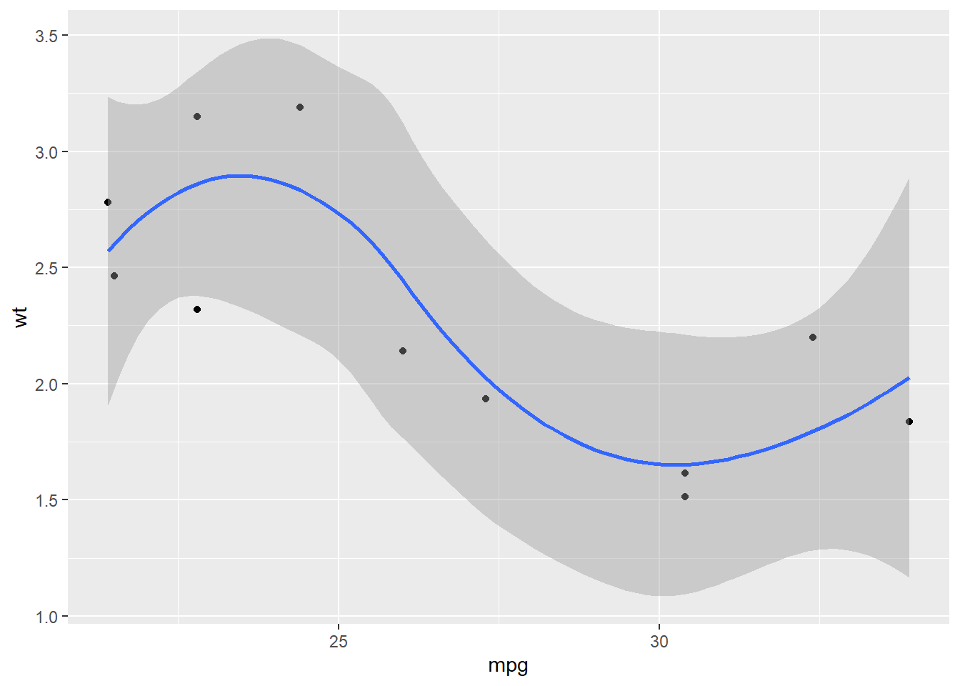
##
## $`6`
## `geom_smooth()` using method = 'loess' and formula 'y ~ x'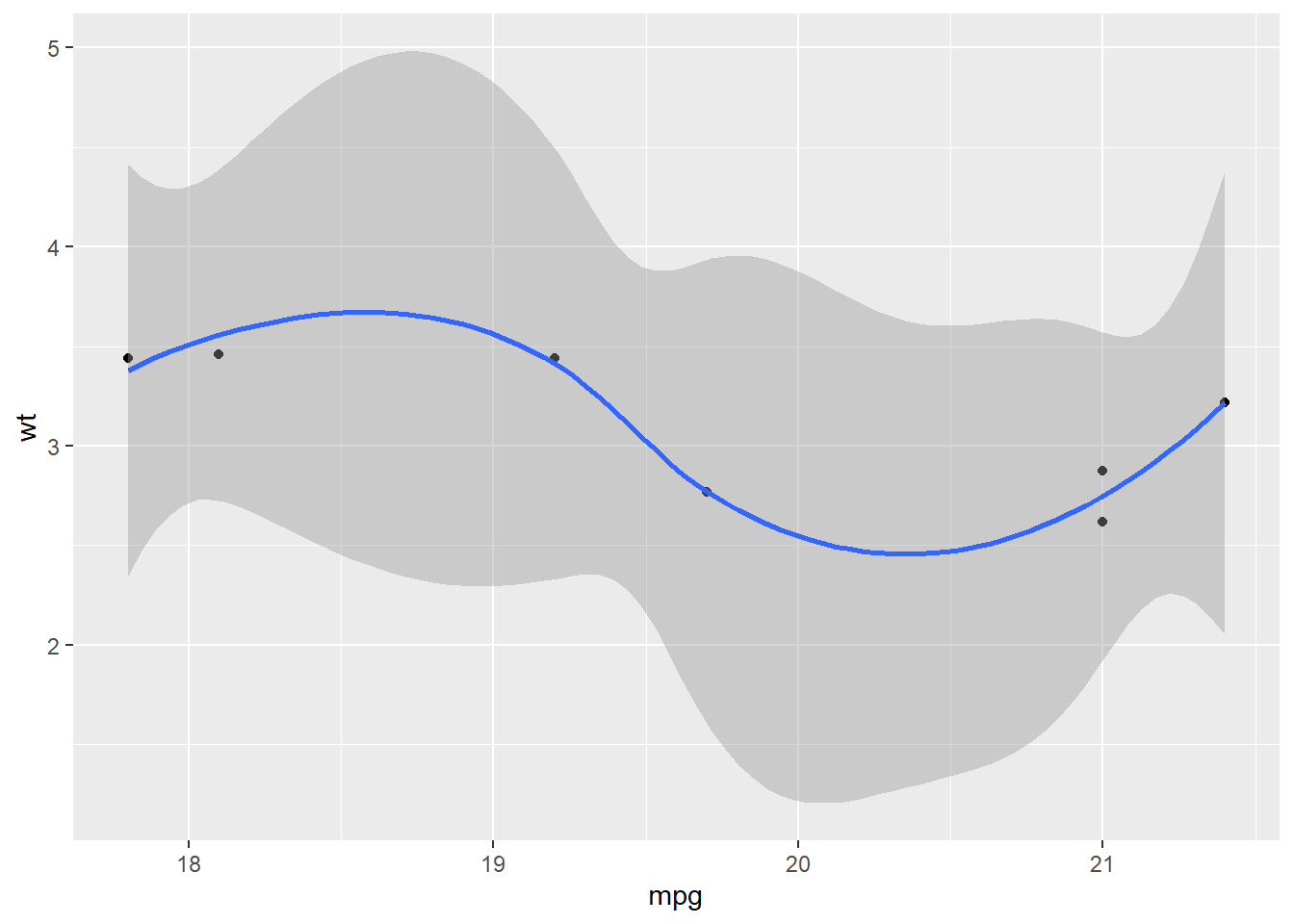
##
## $`8`
## `geom_smooth()` using method = 'loess' and formula 'y ~ x'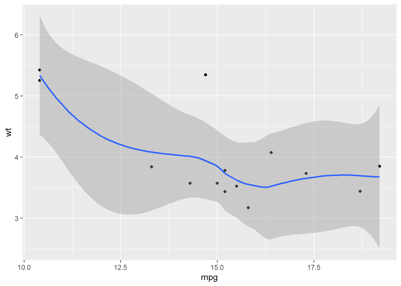
Predicate functions
Purrr also contains functions that check for a condition, so we can set up conditions before iterating.
str(iris)## 'data.frame': 150 obs. of 5 variables:
## $ Sepal.Length: num 5.1 4.9 4.7 4.6 5 5.4 4.6 5 4.4 4.9 ...
## $ Sepal.Width : num 3.5 3 3.2 3.1 3.6 3.9 3.4 3.4 2.9 3.1 ...
## $ Petal.Length: num 1.4 1.4 1.3 1.5 1.4 1.7 1.4 1.5 1.4 1.5 ...
## $ Petal.Width : num 0.2 0.2 0.2 0.2 0.2 0.4 0.3 0.2 0.2 0.1 ...
## $ Species : Factor w/ 3 levels "setosa","versicolor",..: 1 1 1 1 1 1 1 1 1 1 ...iris %>%
map_dbl(mean) # warning, NA for Species## Warning in mean.default(.x[[i]], ...): argument is not numeric or logical:
## returning NA## Sepal.Length Sepal.Width Petal.Length Petal.Width Species
## 5.843333 3.057333 3.758000 1.199333 NAiris %>%
discard(is.factor) %>%
map_dbl(mean) # clean!## Sepal.Length Sepal.Width Petal.Length Petal.Width
## 5.843333 3.057333 3.758000 1.199333starwars %>%
keep(is.character) %>%
map_int(~length(unique(.)))## name hair_color skin_color eye_color sex gender homeworld
## 87 13 31 15 5 3 49
## species
## 38is.factor() and is.character() are examples of “predicate functions”.
To return everything, but apply a function only if a condition is met, we can use map_if():
str(iris)## 'data.frame': 150 obs. of 5 variables:
## $ Sepal.Length: num 5.1 4.9 4.7 4.6 5 5.4 4.6 5 4.4 4.9 ...
## $ Sepal.Width : num 3.5 3 3.2 3.1 3.6 3.9 3.4 3.4 2.9 3.1 ...
## $ Petal.Length: num 1.4 1.4 1.3 1.5 1.4 1.7 1.4 1.5 1.4 1.5 ...
## $ Petal.Width : num 0.2 0.2 0.2 0.2 0.2 0.4 0.3 0.2 0.2 0.1 ...
## $ Species : Factor w/ 3 levels "setosa","versicolor",..: 1 1 1 1 1 1 1 1 1 1 ...iris %>%
map_if(is.numeric, round) %>%
str()## List of 5
## $ Sepal.Length: num [1:150] 5 5 5 5 5 5 5 5 4 5 ...
## $ Sepal.Width : num [1:150] 4 3 3 3 4 4 3 3 3 3 ...
## $ Petal.Length: num [1:150] 1 1 1 2 1 2 1 2 1 2 ...
## $ Petal.Width : num [1:150] 0 0 0 0 0 0 0 0 0 0 ...
## $ Species : Factor w/ 3 levels "setosa","versicolor",..: 1 1 1 1 1 1 1 1 1 1 ...This results in a list in which the elements are rounded only if they store numeric data.
Now, let’s see a more involved example with our climate dataset. In this one, we use functions from dplyr, purrr, stringr, tibble and ggplot2.
# cumulative and yearly change in CO2 emissions dataset
climate_cumul <- climate_tidy %>%
  arrange(`Country name`, year) %>%
  group_by(`Country name`) %>%
  mutate(cumul.CO2.KT = cumsum(EN.ATM.CO2E.KT),
         dif.CO2.KT = EN.ATM.CO2E.KT - lag(EN.ATM.CO2E.KT)) %>%
  map_at(vars(ends_with("KT")), ~ .x / 10^6) %>%
  as_tibble() %>%  # from list to tibble
  rename_at(vars(ends_with("KT")), ~ str_replace(.x, "KT", "PG"))

# visualise it
p <- climate_cumul %>%
  ggplot() +
  aes(x = year,
      y = cumul.CO2.PG,
      colour = `Country name`) +
  geom_line() +
  theme(legend.position = "none")
p
## Warning: Removed 1541 row(s) containing missing values (geom_path).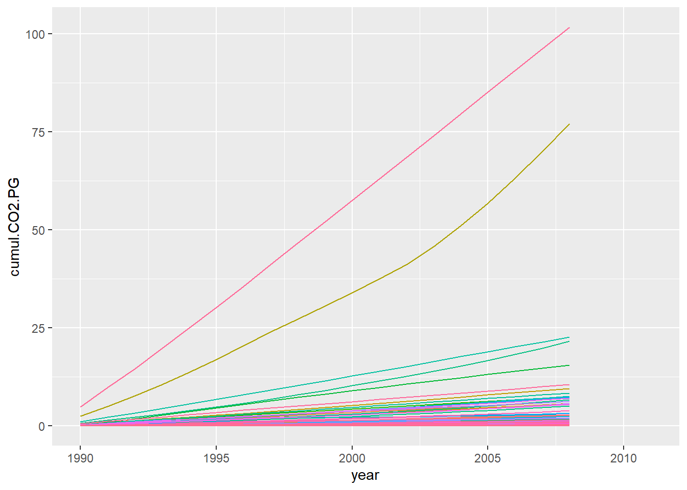
If you want to create an interactive visualisation, you can use plotly:
library(plotly)
ggplotly(p)